Quiz#1 Review Sheet - Question & Answer

/random-numbers.html
Pseudo-Random vs. True RandomThe difference between true random number generators (TRNGs) and pseudo-random number generators (PRNGs) is that TRNGs use an unpredictable physical means to generate numbers (like atmospheric noise), and PRNGs use mathematical algorithms (completely computer-generated).

===============================================

Monte Carlo Integration: Calculating Definite Integrals: (class website)

Pseudorandom Number A slightly archaic term for a computer-generated random number. The prefix pseudo- is used to distinguish this type of number from a "truly" random number generated by a random physical process such as radioactive decay.
==============================================

/randomness/

There are two main approaches to generating random numbers using a computer: Pseudo-Random Number Generators (PRNGs) and True Random Number Generators (TRNGs). The approaches have quite different characteristics and each has its pros and cons.

Pseudo-Random Number Generators (PRNGs)As the word ‘pseudo’ suggests, pseudo-random numbers are not random in the way you might expect, at least not if you're used to dice rolls or lottery tickets. Essentially, PRNGs are algorithms that use mathematical formulae or simply precalculated tables to produce sequences of numbers that appear random. A good example of a PRNG is the linear congruential method. A good deal of research has gone into pseudo-random number theory, and modern algorithms for generating pseudo-random numbers are so good that the numbers look exactly like they were really random.
The basic difference between PRNGs and TRNGs is easy to understand if you compare computer-generated random numbers to rolls of a die. Because PRNGs generate random numbers by using mathematical formulae or precalculated lists, using one corresponds to someone rolling a die many times and writing down the results. Whenever you ask for a die roll, you get the next on the list. Effectively, the numbers appear random, but they are really predetermined. TRNGs work by getting a computer to actually roll the die — or, more commonly, use some other physical phenomenon that is easier to connect to a computer than a die is.
PRNGs are efficient, meaning they can produce many numbers in a short time, and deterministic, meaning that a given sequence of numbers can be reproduced at a later date if the starting point in the sequence is known. Efficiency is a nice characteristic if your application needs many numbers, and determinism is handy if you need to replay the same sequence of numbers again at a later stage. PRNGs are typically also periodic, which means that the sequence will eventually repeat itself. While periodicity is hardly ever a desirable characteristic, modern PRNGs have a period that is so long that it can be ignored for most practical purposes.
These characteristics make PRNGs suitable for applications where many numbers are required and where it is useful that the same sequence can be replayed easily. Popular examples of such applications are simulation and modeling applications. PRNGs are not suitable for applications where it is important that the numbers are really unpredictable, such as data encryption and gambling. It should be noted that even though good PRNG algorithms exist, they aren't always used, and it's easy to get nasty surprises. Take the example of the popular web programming language PHP. If you use PHP for GNU/Linux, chances are you will be perfectly happy with your random numbers. However, if you use PHP for Microsoft Windows, you will probably find that your random numbers aren't quite up to scratch as shown in this visual analysis from 2008. Another example dates back to 2002 when one researcher reported that the PRNG on MacOS was not good enough for scientific simulation of virus infections. The bottom line is that even if a PRNG will serve your application's needs, you still need to be careful about which one you use.
True Random Number Generators (TRNGs) In comparison with PRNGs, TRNGs extract randomness from physical phenomena and introduce it into a computer. You can imagine this as a die connected to a computer, but typically people use a physical phenomenon that is easier to connect to a computer than a die is. The physical phenomenon can be very simple, like the little variations in somebody's mouse movements or in the amount of time between keystrokes. In practice, however, you have to be careful about which source you choose. For example, it can be tricky to use keystrokes in this fashion, because keystrokes are often buffered by the computer's operating system, meaning that several keystrokes are collected before they are sent to the program waiting for them. To a program waiting for the keystrokes, it will seem as though the keys were pressed almost simultaneously, and there may not be a lot of randomness there after all.
===============================================

BasicsOfMonteCarloSimulations.doc (class website)

* Computer-generated numbers aren't really random, since computers are deterministic. But, given a number to start with--generally called a random number seed--a number of mathematical operations can be performed on the seed so as to generate unrelated (pseudorandom) numbers. The output of random number generators is tested with rigorous statistical tests to ensure that the numbers are random in relation to one another. One caveat: If you use a random number seed more than once, you will get identical random numbers every time. Thus, for multiple trials, different random number seeds must be used. Commercial programs, like Mathematica, pull a random number seed from somewhere within the system--perhaps the time on the clock--so the seed is unlikely to be the same for two different experiments.

Note: The above Astrix statement was taking from the following:

Note: (from the BasicsOfMonteCarloSimulations.doc)
"Hit and miss" integration is the simplest type of MC method to understand, and it is the type of experiment used in this lab to determine the HCl/DCl energy level population distribution. Before discussing the lab, however, we will begin with a simple geometric MC experiment which calculates the value of pi based on a "hit and miss" integration. Monte Carlo Calculation of Pi
If we say our circle's radius is 1.0, for each throw we can generate two random numbers, an x and a y coordinate, which we can then use to calculate the distance from the origin (0,0) using the Pythagorean theorem. If the distance from the origin is less than or equal to 1.0, it is within the shaded area and counts as a hit. Do this thousands (or millions) of times, and you will wind up with an estimate of the value of pi. How good it is depends on how many iterations (throws) are done, and to a lesser extent on the quality of the random number generator. Simple computer code for a single iteration, or throw, might be: x=(random#) y=(random#) dist=sqrt(x^2 + y^2) if dist.from.origin (less.than.or.equal.to) 1.0 let hits=hits+1.0

Wiki Source: (Using Monte Carlo Method)

For example, consider a circle inscribed in a square. Given that the circle and the square have a ratio of areas that is π/4, the value of π can be approximated using a Monte Carlo method: ^{(4 STEPS BELOW)}

1. 
   
2. 1) Draw a square on the ground, then inscribe a circle within it.
3. 2) Uniformly scatter some objects of uniform size (grains of rice or sand) over the square.
4. 3) Count the number of objects inside the circle and the total number of objects.
5. 4) The ratio of the two counts is an estimate of the ratio of the two areas, which is π/4. Multiply the result by 4 to estimate π.

In this procedure the domain of inputs is the square that circumscribes our circle. We generate random inputs by scattering grains over the square then perform a computation on each input (test whether it falls within the circle). Finally, we aggregate the results to obtain our final result, the approximation of π.
To get an accurate approximation for π this procedure should have two other common properties of Monte Carlo methods.

First, the inputs should truly be random. If grains are purposefully dropped into only the center of the circle, they will not be uniformly distributed, and so our approximation will be poor.

Second, there should be a large number of inputs. The approximation will generally be poor if only a few grains are randomly dropped into the whole square. On average, the approximation improves as more grains are dropped.
===============================================

More from Wiki:

Monte Carlo methods vary, but tend to follow a particular pattern:

1. 1) Define a domain of possible inputs.
2. 2) Generate inputs randomly from a probability distribution over the domain.
3. 3) Perform a deterministic computation on the inputs.
4. 4) Aggregate the results.

Wiki Source:

In numerical analysis, numerical integration constitutes a broad family of algorithms for calculating the numerical value of a definite integral, and by extension, the term is also sometimes used to describe the numerical solution of differential equations. This article focuses on calculation of definite integrals. The term numerical quadrature (often abbreviated to quadrature) is more or less a synonym for numerical integration, especially as applied to one-dimensional integrals. Numerical integration over more than one dimension is sometimes described as cubature,^[1] although the meaning of quadrature is understood for higher dimensional integration as well. The basic problem considered by numerical integration is to compute an approximate solution to a definite integral: If f(x) is a smooth well-behaved function, integrated over a small number of dimensions and the limits of integration are bounded, there are many methods of approximating the integral with arbitrary precision.
Reasons for numerical integration There are several reasons for carrying out numerical integration. The integrand f(x) may be known only at certain points, such as obtained by sampling. Some embedded systems and other computer applications may need numerical integration for this reason. A formula for the integrand may be known, but it may be difficult or impossible to find an antiderivative which is an elementary function. An example of such an integrand is f(x) = exp(−x²), the antiderivative of which (the error function, times a constant) cannot be written in elementary form. It may be possible to find an antiderivative symbolically, but it may be easier to compute a numerical approximation than to compute the antiderivative. That may be the case if the antiderivative is given as an infinite series or product, or if its evaluation requires a special function which is not available.

FINAL ANSWER (GO WITH THIS)!!!!!!!!

A time series is point data at time intervals.

(answer came from June 7th Lecture Notes)

==============================================

/div898/handbook/pmc/section4/pmc4.htm

Time series analysis accounts for the fact that data points taken over time may have an internal structure (such as autocorrelation, trend or seasonal variation) that should be accounted for.

==============================================

/terms/t/timeseries.asp#axzz1PsyEKLGj

What Does Time Series Mean?
A sequence of numerical data points in successive order, usually occurring in uniform intervals. In plain English, a time series is simply a sequence of numbers collected at regular intervals over a period of time.

==============================================

Wiki Source: (http://en.wikipedia.org/wiki/Time_series)

A time series is a sequence of data points, measured typically at successive times spaced at uniform time intervals. Examples of time series are the daily closing value of the Dow Jones index or the annual flow volume of the Nile River at Aswan.

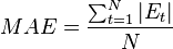
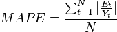
MAE (Mean Absolute Error) - Sum of the magnitude (abs. value) of errors divided by N. (Average Absolute Error). MAPE (Mean Absolute Percentage Error) - Sum of the Error – Average of - [Error/Actual Value] MSE (Mean Square Error) - Average of sum of the Errors squared. [Looks somewhat like Standard Deviation]. Quantitative Forecasting Techniques 1. (Educated) Guessing 2. Last Period Technique 3. Moving Averages (Something we can compute) Time Series Example: Period Value Moving Average Error 1 100 No Error 2 102 No Error 3 99 No Error 4 97 *5 89 99.25 -10.25 6 103 96.75 6.25 7 104 8 102 9 99 10 104 11 102 12 105 13 111 Moving Average: 4 day moving avg: Day #5: (100+102+99+97)/4 = 99.25 Our prediction for day 5 … I was 89! We was wrong! Day #6: (102+99+97+89)/4 = 387/4 = 96.75 MAE = Sum Errors / 9 Advantages + Disadvantages of Spreadsheet Solution to Moving Average. Adv. 1. Fast 2. Accurate Enough 3. Easy to understand output format (rows and columns) 4. Easy to graph solution. Dis. 1. Distribution 2. Difficult to expand 3. Error checking C++ has stl standard template library (STL Library). Must have dynamic arrays to do this problem. So write it in Python or PHP because they have dynamic arrays (arrays that will change in size). Input Data Create Size Input N (number of data points in moving average) N = 5 0,1,2,3,4 For (int I = N – 1; I <= size – 1; I++){ · ß 1) *Sum should be an array and compared in a loop. 2) All this is great! Problem is size of this array. Create sum of data points Div. by N Write to output array } Print output;
Wiki Source - Moving Averages:
Given a series of numbers and a fixed subset size, the moving average can be obtained by first taking the average of the first subset. The fixed subset size is then shifted forward, creating a new subset of numbers, which is averaged. This process is repeated over the entire data series. The plot line connecting all the (fixed) averages is the moving average. A moving average is a set of numbers, each of which is the average of the corresponding subset of a larger set of data points. A moving average may also use unequal weights for each data value in the subset to emphasize particular values in the subset.
A moving average is commonly used with time series data to smooth out short-term fluctuations and highlight longer-term trends or cycles. The threshold between short-term and long-term depends on the application, and the parameters of the moving average will be set accordingly. For example, it is often used in technical analysis of financial data, like stock prices, returns or trading volumes. It is also used in economics to examine gross domestic product, employment or other macroeconomic time series. Mathematically, a moving average is a type of convolution and so it can be viewed as an example of a low-pass filter used in signal processing.

When used with non-time series data, a moving average filters higher frequency components without any specific connection to time, although typically some kind of ordering is implied. Viewed simplistically it can be regarded as smoothing the data.

Note: There are several types of moving averages. Such as simple, cumulative, weighted, exponential, and modified. I will focus on simple moving average example.
Simple moving average In financial applications a simple moving average (SMA) is the unweighted mean of the previous n data points.^[1] However, in science and engineering the mean is normally taken from an equal number of data either side of a central value. This ensures that variations in the mean are aligned with the variations in the data rather than being shifted in time. An example of a simple unweighted running mean for a 10-day sample of closing price is the mean of the previous 10 days' closing prices. If those prices are then the formula is When calculating successive values, a new value comes into the sum and an old value drops out, meaning a full summation each time is unnecessary for this simple case, The period selected depends on the type of movement of interest, such as short, intermediate, or long term. In financial terms moving average levels can be interpreted as resistance in a rising market, or support in a falling market. If the data used is not centred around the mean, a simple moving average lags behind the latest data point by half the sample width. A SMA can also be disproportionately influenced by old data points dropping out or new data coming in. One characteristic of the SMA is that if the data have a periodic fluctuation, then applying an SMA of that period will eliminate that variation (the average always containing one complete cycle). But a perfectly regular cycle is rarely encountered.^[2] For a number of applications it is advantageous to avoid the shifting induced by using only 'past' data. Hence a central moving average can be computed, using data equally spaced either side of the point in the series where the mean is calculated. This requires using an odd number of data points in the sample window.
==============================================Another Example of Moving Averages
http://stockcharts.com/school/doku.php?id=chart_school:technical_indicators:moving_averages

Moving Averages Introduction Moving averages smooth the price data to form a trend following indicator. They do not predict price direction, but rather define the current direction with a lag. Moving averages lag because they are based on past prices. Despite this lag, moving averages help smooth price action and filter out the noise. They also form the building blocks for many other technical indicators and overlays, such as Bollinger Bands, MACD and the McClellan Oscillator. The two most popular types of moving averages are the Simple Moving Average (SMA) and the Exponential Moving Average (EMA). These moving averages can be used to identify the direction of the trend or define potential support and resistance levels. SMA Calculation A simple moving average is formed by computing the average price of a security over a specific number of periods. Most moving averages are based on closing prices. A 5-day simple moving average is the five day sum of closing prices divided by five. As its name implies, a moving average is an average that moves. Old data is dropped as new data comes available. This causes the average to move along the time scale. Below is an example of a 5-day moving average evolving over three days. Daily Closing Prices: 11,12,13,14,15,16,17 First day of 5-day SMA: (11 + 12 + 13 + 14 + 15) / 5 = 13 Second day of 5-day SMA: (12 + 13 + 14 + 15 + 16) / 5 = 14 Third day of 5-day SMA: (13 + 14 + 15 + 16 + 17) / 5 = 15 The first day of the moving average simply covers the last five days. The second day of the moving average drops the first data point (11) and adds the new data point (16). The third day of the moving average continues by dropping the first data point (12) and adding the new data point (17). In the example above, prices gradually increase from 11 to 17 over a total of seven days. Notice that the moving average also rises from 13 to 15 over a three day calculation period. Also notice that each moving average value is just below the last price. For example, the moving average for day one equals 13 and the last price is 15. Prices the prior four days were lower and this causes the moving average to lag.

Wiki Source: (before we look at forecasting accuracy ... let's look at what forecasting is first).
Forecasting is the process of making statements about events whose actual outcomes (typically) have not yet been observed. A commonplace example might be estimation for some variable of interest at some specified future date. Prediction is a similar, but more general term. Both might refer to formal statistical methods employing time series, cross-sectional or longitudinal data, or alternatively to less formal judgemental methods. Usage can differ between areas of application: for example in hydrology, the terms "forecast" and "forecasting" are sometimes reserved for estimates of values at certain specific future times, while the term "prediction" is used for more general estimates, such as the number of times floods will occur over a long period. Risk and uncertainty are central to forecasting and prediction; it is generally considered good practice to indicate the degree of uncertainty attaching to forecasts.

The process of climate change and increasing energy prices has led to the usage of Egain Forecasting of buildings. The method uses Forecasting to reduce the energy needed to heat the building, thus reducing the emission of greenhouse gases. Forecasting is used in the practice of Customer Demand Planning in every day business forecasting for manufacturing companies. The discipline of demand planning, also sometimes referred to as supply chain forecasting, embraces both statistical forecasting and a consensus process. An important, albeit often ignored aspect of forecasting, is the relationship it holds with planning. Forecasting can be described as predicting what the future will look like, whereas planning predicts what the future should look like. There is no single right forecasting method to use. Selection of a method should be based on your objectives and your conditions (data etc.). A good place to find a method, is by visiting a selection tree. An example of a selection tree can be found here.
===============================================

Note: (the 4 aspects of this that we need to know are listed below; ex: MAE, MAPE, PMAD, MSE, and RMSE - pick 4 out of the 6 possible aspects/options)

Forecasting accuracy The forecast error is the difference between the actual value and the forecast value for the corresponding period. where E is the forecast error at period t, Y is the actual value at period t, and F is the forecast for period t. Measures of aggregate error: Mean Absolute Error (MAE) Mean Absolute Percentage Error (MAPE) Percent Mean Absolute Deviation (PMAD) Mean squared error (MSE) Root Mean squared error (RMSE) Forecast skill (SS) Please note that business forecasters and practitioners sometimes use different terminology in the industry. They refer to the PMAD as the MAPE, although they compute this volume weighted MAPE. For more information see Calculating Demand Forecast Accuracy Reference class forecasting was developed to increase forecasting accuracy.
Applications of forecasting Forecasting has application in many situations:

• Supply chain management - Forecasting can be used in Supply Chain Management to make sure that the right product is at the right place at the right time. Accurate forecasting will help retailers reduce excess inventory and therefore increase profit margin. Accurate forecasting will also help them meet consumer demand.
• Weather forecasting, Flood forecasting and Meteorology
• Transport planning and Transportation forecasting
• Economic forecasting
• Egain Forecasting
• Technology forecasting
• Earthquake prediction
• Land use forecasting
• Product forecasting
• Player and team performance in sports
• Telecommunications forecasting
• Political Forecasting
• Sales Forecasting

(Write the definition Write an example Be able to identify each of the 5 terms)

A class is an expanded concept of a data structure: instead of holding only data, it can hold both data and functions.

An object is an instantiation of a class. In terms of variables, a class would be the type, and an object would be the variable.

Classes are generally declared using the keyword class, with the following format:

class class_name { access_specifier_1: member1; access_specifier_2: member2; ... } object_names;

Definition: In C++ and C#, classes can be defined as deriving from a base class. A derived class inherits all of the ancestors protected and public methods and data members. With inheritance if a method is made virtual in the base class then the derived class can override it with different behaviour. This makes possible polymorphism.
==============================================
Inheritance is a mechanism of reusing and extending existing classes without modifying them, thus producing hierarchical relationships between them. Inheritance is almost like embedding an object into a class. Suppose that you declare an object x of class A in the class definition of B. As a result, class B will have access to all the public data members and member functions of class A. However, in class B, you have to access the data members and member functions of class A through object x. The following example demonstrates this: #include using namespace std; class A { int data; public: void f(int arg) { data = arg; } int g() { return data; } }; class B { public: A x; }; int main() { B obj; obj.x.f(20); cout << obj.x.g() << endl; // cout << obj.g() << endl; }

=================================================

Lets say we have two classes. A and B. Class B inherits from class A. 01#include 02 03using namespace std;04 05class A06{07public:08 A() { a_member = 0; }09 int a_member;10};11 12class B : public A13{14public:15 B() : A() { b_member = 0; };16 int b_member;17};18 19int main()20{21 A *a = new B;22 a->a_member = 10;23 24 return 0;25} The interesting thing to notice here is that a actually points to instance of class B. When dereferencing a_member, we’re actually dereferencing a_member that defined in class A, but belongs to class B (via inheritance). To make this happen, compiler has to make sure that common part of both classes (a_member in our case) located at the same offset in the object.

Composition is a relationship between two classes that is based on the aggregation relationship. Composition takes the relationship one step further by ensuring that the containing object is responsible for the lifetime of the object it holds. If Object B is contained within Object A, then Object A is responsible for the creation and destruction of Object B. Unlike aggregation, Object B cannot exist without Object A.

Example of Composition (from class):
*add 'Composition' to Shape class
class geoCenter {
private: float x, y;
public:
geoCenter (float x, float y) {
this -> x=x'
this -> y=y;

void setCenter ( );

float getX {return x;}
float getY {return y;}
}

Add to Shape class to make composition (below):

protected:
int givenSize;
geoCenter * origin; //this is a pointer to array

constructor:
Shape{
origin new GeoCenter (0, 0);
}

To Use It:
1) Set center (i, 2i) -- after you instantiate square or cirlce.
2) In 3rd loop, also print center coordinates.

Define:
Polymorphism - refers to a programming language's ability to process objects differently depending on their data type or class. More specifically, it is the ability to redefine methods for derived classes. For example, given a base class shape, polymorphism enables the programmer to define different area methods for any number of derived classes, such as circles, rectangles and triangles. No matter what shape an object is, applying the area method to it will return the correct results. Polymorphism is considered to be a requirement of any true object-oriented programming language (OOPL).

===============================================

How basic polymorphism worksBACK TO TOC Let’s change our example a bit and add some virtual methods. 01#include 02 03using namespace std;04 05class A06{07public:08 A() { a_member = 0; }09 virtual int reset() { a_member = 0; }10 void set_a_member( int a ) { a_member = a; }11 int get_a_member() { return a_member; }12protected:13 int a_member;14};15 16class B : public A17{18public:19 B() : A() { b_member = 0; };20 virtual int reset() { a_member = b_member = 0; }21 virtual void some_virtual_method() { }22 void set_b_member(int b ) { b_member = b; }23 int get_b_member() { return b_member; }24protected:25 int b_member;26};27 28int main()29{30 B *b = new B;31 A *a = b;32 33 b->set_b_member( 20 );34 b->set_a_member( 10 );35 36 a->reset();37 38 cout << b->get_a_member() << " " << b->get_b_member() <<39 endl;40 41 return 0;42} If you compile and run this program it will obviously print “0 0″. But how, you may ask. After all we did a->reset(). Without our understanding of polymorphism we could think that we’re calling method that belongs to class A. The reason it works is because when compiler sees code that dereferences pointer to A it expects certain internal object structure and when it dereferences pointer to B it expects different object structure. Let us take a look at both of them. However even more important here is the structure of the virtual methods tables of both classes. It is because of the virtual methods table structure compilers knows what virtual method to call. When it generates the code that dereferences pointer to A, it expects that first method in the virtual methods table of the object will be pointer to right reset() routine. It doesn’t really care if the pointer actually points to B object. It will call first method of the virtual methods table anyway.

Define:
Abstract Class - Has virtual methods you implement in a derived class.

==============================================

more on abstract classes ...
An abstract class is a class that is designed to be specifically used as a base class. An abstract class contains at least one pure virtual function. You declare a pure virtual function by using a pure specifier (= 0) in the declaration of a virtual member function in the class declaration.
The following is an example of an abstract class:
class AB { public: virtual void f() = 0; };Function AB::f is a pure virtual function. A function declaration cannot have both a pure specifier and a definition. For example, the compiler will not allow the following: struct A { virtual void g() { } = 0; };

Define:
Interface - A list of methods you implement.

================================================

more on interface ...
A boundary across which two independent systems meet and act on or communicate with each other. In computer technology, there are several types of interfaces.

• user interface - the keyboard, mouse, menus of a computer system. The user interface allows the user to communicate with the operating system. Also see GUI.
• software interface - the languages and codes that the applications use to communicate with each other and with the hardware.
• hardware interface - the wires, plugs and sockets that hardware devices use to communicate with each other.

(v.) To connect with or interact with by means of an interface.

Sequential Files Sequential file techniques provide a straightforward way to read and write files. PowerBASIC's sequential file commands manipulate text files: files of ANSI or WIDE characters with carriage-return/linefeed pairs separating records.
Quite possibly, the best reason for using sequential files is their degree of portability to other programs, programming languages, and computers. Because of this, you can often look at sequential files as the common denominator of data processing, since they can be read by word-processing programs and editors (such as PowerBASIC's), absorbed by other applications (such as database managers), and sent over the Internet to other computers.
The idea behind sequential files is simplicity itself: write to them as though they were the screen and read from them as though they were the keyboard.

Create a sequential file using the following steps:

1. 
   
2. Open the file in sequential output mode. To create a file in
   
3. 
   
4. PowerBASIC, you must use the OPEN statement. Sequential files have two options to prepare a file for output:

OUTPUT: If a file does not exist, a new file is created. If a file already exists, its contents are erased, and the file is then treated as a new file. APPEND: If a file does not exist, a new file is created. If a file already exists, PowerBASIC appends (adds) data at the end of that file.

2. 
   
3. Output data to a file. Use WRITE# or PRINT# to write data to a sequential file.
4. 
   
5. Close the file. The CLOSE statement closes a file after the program has completed all I/O operations.

======================
To read a sequential file:

1. First, OPEN the file in sequential INPUT mode. This prepares the file for reading.
2. 
   
3. Read data in from the file. Use PowerBASIC's INPUT# or LINE INPUT# statements.
4. 
   
5. Close the file. The CLOSE statement closes a file after the program has completed all I/O operations.

The drawback to sequential files is, not surprisingly, that you only have sequential access to your data. You access one line at a time, starting with the first line. This means if you want to get to the last line in a sequential file of 23,000 lines, you will have to read the preceding 22,999 lines. Sequential files, therefore, are best suited to applications that perform sequential processing (for example, counting words, checking spelling, printing mailing labels in file order) or in which all the data can be held in memory simultaneously. This allows you to read the entire file in one fell swoop at the start of a program and to write it all back at the end. In between, the information can be stored in an array (in memory) which can be accessed randomly. Although the SEEK statement can be used to change the point in the file where the next read or write will occur, the calculations required to determine the position of the start of each record in a sequential file would add considerable overhead. Sequential files typically consist of records of varying sizes. Either you would have to maintain a separate index file indicating the starting byte position of each record, or you would have to seek randomly until you found the correct position. However, SEEK does have its uses with sequential files. For instance, after reading an entire file, you could use SEEK to reposition the file pointer to the start of the file, in order to process the data a second time. This is certainly quicker than closing and re-opening the file. Sequential files lend themselves to database situations in which the length of individual records is variable. For example, suppose an alumni list had a comments field. Some people may have 100 bytes or more of comments. Others, perhaps most, will have none. Sequential files handle this problem without wasting disk space.
The OPEN statement provides an optional LEN parameter for use with sequential files. This instructs PowerBASIC to use internal buffering to speed up reading of sequential files, using a buffer of the size specified by the LEN parameter. A buffer of 8192 bytes is suggested for best general performance, especially when networks are involved. However, this value can be increased in size to gain additional performance - the best value will always be specific to a particular combination of hardware and software, and may vary considerably from PC to PC, network to network, etc.
The OPEN statement also provides an optional character mode parameter. This specifies the character mode for this file: ANSI or WIDE (Unicode). Since sequential files consist of text alone, the selected mode is enforced by PowerBASIC. All data read or written to the file is automatically forced to the selected mode, regardless of the type of variables or expressions used. With binary or random files, this specification has no effect, but it may be included in your code for self-documentation purposes. ANSI characters in the U.S. range of CHR$(0) to CHR$(127) are known as ASCII, and are always represented by a single byte. International ANSI characters in the range of CHR$(128) to CHR$(255) may be followed by one or more additional bytes in order to accurately represent non-U.S. characters. The exact definition of these characters depends upon the character set in use. WIDE characters are always represented by two bytes per character. If the Chr option is not specified, the default mode is ANSI.

(SAME AS ABOVE)

Sequential Files Sequential file techniques provide a straightforward way to read and write files. PowerBASIC's sequential file commands manipulate text files: files of ANSI or WIDE characters with carriage-return/linefeed pairs separating records.
Quite possibly, the best reason for using sequential files is their degree of portability to other programs, programming languages, and computers. Because of this, you can often look at sequential files as the common denominator of data processing, since they can be read by word-processing programs and editors (such as PowerBASIC's), absorbed by other applications (such as database managers), and sent over the Internet to other computers.
The idea behind sequential files is simplicity itself: write to them as though they were the screen and read from them as though they were the keyboard.

Create a sequential file using the following steps:

1. 
   
2. Open the file in sequential output mode. To create a file in
   
3. 
   
4. PowerBASIC, you must use the OPEN statement. Sequential files have two options to prepare a file for output:

OUTPUT: If a file does not exist, a new file is created. If a file already exists, its contents are erased, and the file is then treated as a new file. APPEND: If a file does not exist, a new file is created. If a file already exists, PowerBASIC appends (adds) data at the end of that file.

2. 
   
3. Output data to a file. Use WRITE# or PRINT# to write data to a sequential file.
4. 
   
5. Close the file. The CLOSE statement closes a file after the program has completed all I/O operations.

======================
To read a sequential file:

1. First, OPEN the file in sequential INPUT mode. This prepares the file for reading.
2. 
   
3. Read data in from the file. Use PowerBASIC's INPUT# or LINE INPUT# statements.
4. 
   
5. Close the file. The CLOSE statement closes a file after the program has completed all I/O operations.

The drawback to sequential files is, not surprisingly, that you only have sequential access to your data. You access one line at a time, starting with the first line. This means if you want to get to the last line in a sequential file of 23,000 lines, you will have to read the preceding 22,999 lines. Sequential files, therefore, are best suited to applications that perform sequential processing (for example, counting words, checking spelling, printing mailing labels in file order) or in which all the data can be held in memory simultaneously. This allows you to read the entire file in one fell swoop at the start of a program and to write it all back at the end. In between, the information can be stored in an array (in memory) which can be accessed randomly. Although the SEEK statement can be used to change the point in the file where the next read or write will occur, the calculations required to determine the position of the start of each record in a sequential file would add considerable overhead. Sequential files typically consist of records of varying sizes. Either you would have to maintain a separate index file indicating the starting byte position of each record, or you would have to seek randomly until you found the correct position. However, SEEK does have its uses with sequential files. For instance, after reading an entire file, you could use SEEK to reposition the file pointer to the start of the file, in order to process the data a second time. This is certainly quicker than closing and re-opening the file. Sequential files lend themselves to database situations in which the length of individual records is variable. For example, suppose an alumni list had a comments field. Some people may have 100 bytes or more of comments. Others, perhaps most, will have none. Sequential files handle this problem without wasting disk space.
The OPEN statement provides an optional LEN parameter for use with sequential files. This instructs PowerBASIC to use internal buffering to speed up reading of sequential files, using a buffer of the size specified by the LEN parameter. A buffer of 8192 bytes is suggested for best general performance, especially when networks are involved. However, this value can be increased in size to gain additional performance - the best value will always be specific to a particular combination of hardware and software, and may vary considerably from PC to PC, network to network, etc.
The OPEN statement also provides an optional character mode parameter. This specifies the character mode for this file: ANSI or WIDE (Unicode). Since sequential files consist of text alone, the selected mode is enforced by PowerBASIC. All data read or written to the file is automatically forced to the selected mode, regardless of the type of variables or expressions used. With binary or random files, this specification has no effect, but it may be included in your code for self-documentation purposes. ANSI characters in the U.S. range of CHR$(0) to CHR$(127) are known as ASCII, and are always represented by a single byte. International ANSI characters in the range of CHR$(128) to CHR$(255) may be followed by one or more additional bytes in order to accurately represent non-U.S. characters. The exact definition of these characters depends upon the character set in use. WIDE characters are always represented by two bytes per character. If the Chr option is not specified, the default mode is ANSI.